Introduction to R
R is a programming language for analytical computing and presentation. It is a GNU project which is similar to the S language and environment which was developed by John Chambers and colleagues at Bell Laboratories (formerly AT&T, now Nokia Bell Labs). R can be considered as a different implementation of S.
"
R is an official part of the Free Software Foundation’s GNU project, and the
R Foundation has similar goals to other open source software foundations like the Apache Foundation or the GNOME Foundation."
One of R’s strengths is the ease of use combined with enormous expressive and programming production power.
R runs on a wide variety of UNIX/Linux platforms, Windows and MacOS X.
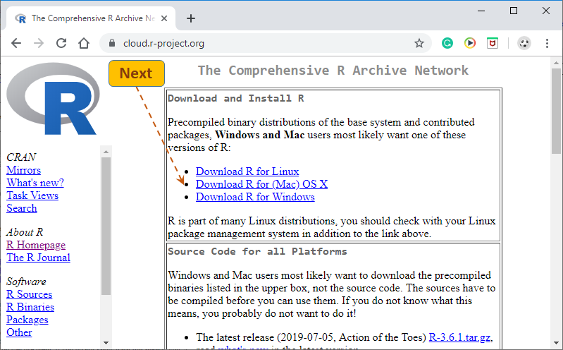
On the next page, in the 0-Cloud section, select the first link.
Depending on your OS, select (download) the appropriate R setup options. The remaining part of this instruction will use the Windows installer.
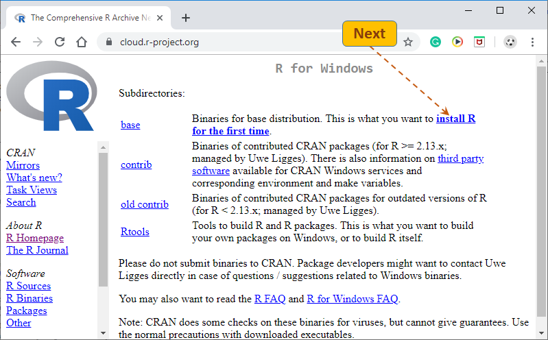
Most likely, you will need to follow the "
install R for the first time" link. Click
here if you want to upgrade your existing
R installation.
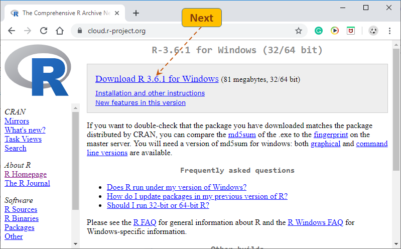
Finally, click the Download R … link (this option is for the Windows OS).
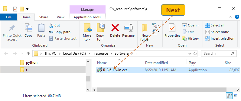
On the instructor's system, the setup program was downloaded to folder C:/_resource/software/R. Notice that R uses forward slash (/) as a directory separator also on Windows.
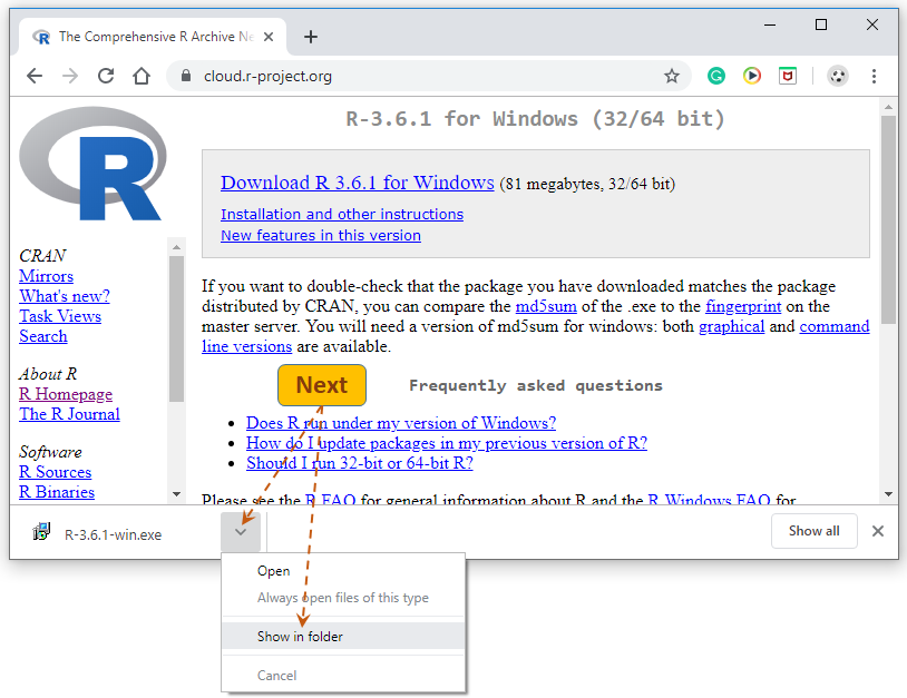
Another popular destination is just the Windows' Download folder. Acutely, with Google Chrome, we can go directly to this folder by following the download path as shown below.
Next, launch (double-click) the setup program.
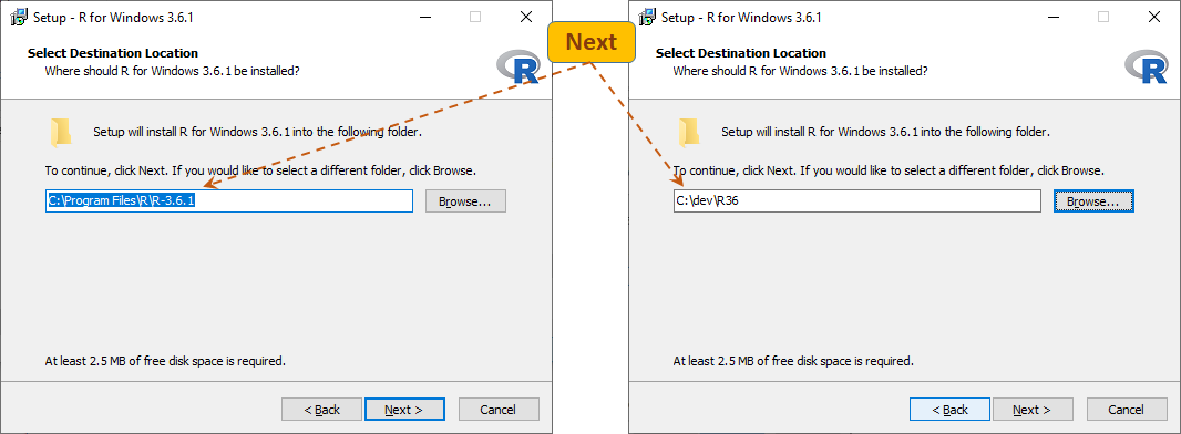
The installation process is simple. I would only suggest changing the installation's target folder.
When you get to the folder setup form, you may wish to change the installation folder to a simpler target, for example to C:\dev\R36
(no need to make any changes on Mac). In this instruction the installation folder of R (here C:/dev/R36) will be referred to as %rhome%.
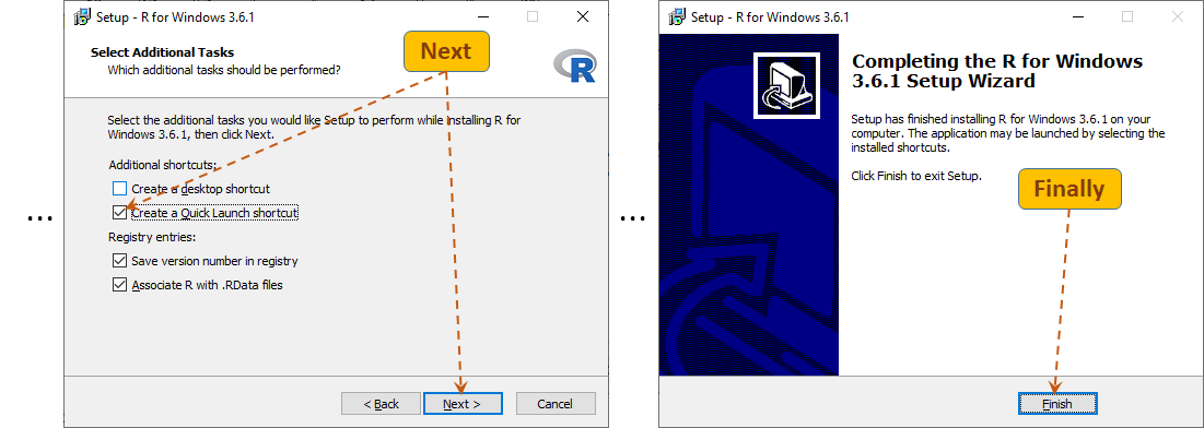
From this point on, just click the
Next buttons (except maybe for adding an
R shortcut to the
Quick Lunch bar.) and the last
Finish button.
Additional Installation Procedures
In addition to the powerful functionality provided by the basic R installation, many users and organization have developed convenient libraries that can be incorporated into our R environment.
For example, you may recall the data structure for ANOVA that you used in Excel. In R, the same data set that is good for Excel must be reorganized (reshaped). Library "reshape2" provides an easy to use function called melt(). This function will become available after the following library has been installed:
install.packages("reshape2")
This installation uses the default library location that was created by the R installer. On your instructor's computer, this location (folder) is: %rhome%/library (here C:\dev\R36\library).
If you also installed R within the Anaconda distribution, this location will be different. On the instructor's computer, Anaconda is installed in directory C:/dev/anaconda. Let's refer to it as %ANACONDA_HOME%. Within this installation, the R library's folder is:
%ANACONDA_HOME%/Lib/R/library (here C:/dev/anaconda/Lib/R/library).
The following example shows how to install two libraries ("pckg1" and "pckg2") at this location:
install.packages(c("pckg1", "pckg2"), lib="C:/dev/anaconda/Lib/R/library")
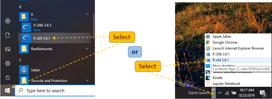
Find R in and lunch it from the Start list or use the Quick Lunch pop-up to locate and lunch R. These shortcuts lead to program R GUI (Rgui.exe) that is located in the bin/x64 subfolder of the R Home folder (here C:/dev/R36). This is a Graphical User Interface version of R. By the way, this instruction assumes that you are using a 64-bit operating systems. It is also possible to run R GUI in its 32-bit mode (from folder bin/i386).
If you prefer to have a shortcut to R GUI on your desktop, open folder C:/dev/R36\bin/x64, Copy file Rgui.exe and paste it as shortcut on the desktop. If you installed R in a different folder, go to that folder, find subfolder bin/x64 and program Rgui.exe there. Whichever method you use, R will open its GUI (Graphical User Interface) window with R Console filled with messages and ready for work:
You may wish to press Ctrl+L to clear the messages and write a few lines of code, for example:
a = 3
b = -2
c = -8
Suppose that the three variables hold the values of the parameters of a quadratic equation (ax2+bx+c = 0). One way to solve this equations is to first calculate the discriminant of the equation:
discr = b^2 -4*a*c
discr
[1] 100
Since the value of the discriminant is positive, the equation has two different roots:
sd = sqrt(discr)
twoa = 2 * a
x1 = (-b - sd) / twoa
x2 = (-b + sd) / twoa
x1
[1] -1.333333
x2
[1] 2
The roots (x1, x2) of this equation are (1.333333, 2). Enter q() to quit R GUI. Since you can reuse the above code to run this application again, you may wish to press No.
R [Plain] Console
It is also possible to run [plain] R in a Command (Console) window. Just execute program R.exe from directory %rhome%/bin
(here C:/dev/R36/bin):
R opens an interactive Console that is similar to the R GUI's Console but there are no menu options. The following example shows a simple work done in such a Console. It calculates the monthly loan payment given the principal (present) value of the loan (p), periodic interest rate (r), and the number of payments (n). The loan amount is caclulates according to the following formula:
Notice that the original input for the rate and term is given on the annual basis.
R can also be lunched from a Power Shell window. In File Explorer, hold down Shift, point to and right-click subfolder bin in folder %R_HOME% (here C:\dev\R36). From the popup menu, select option Open
Windows open a Power Shell console. To run R, just enter .\R. An R console opens. It is similar to the Rterm (R-terminal) window shown above. Notice that in the Power Shell, the R command is preceded by token .\ which tells Windows to run R from the current directory (.\). Try some R code, for example check multiplication vs. exponentiation, and quit R without saving this session. Do not close the Power Shell window.
It would appear that the plain R consoles are not worth any attention. However, there are circumstances when running R, for example, from a Power Shell window is advantageous. Let go back to our loan payment example. This time, we will write and save the code in a plain text document, pmt.r. Open a text editor (Notepad) and type the following lines of code.
arg = commandArgs(TRUE)
principal = as.numeric(arg[1])
annual_rate = as.numeric(arg[2])
years = as.numeric(arg[3])
r = annual_rate / 12
n = years * 12
pmt = r * principal / (1 - (1 + r)^-n)
print("Monthly Payement:")
print(round(pmt,2))
Save this document in a folder dedicated to R, for example in C:\dev\rapp\ as pmt.r. Back in the Power Shell window, enter the following command:
./Rscript C:/dev/rapp/pmt.r 100000 0.06 15
This command invokes program Rscript.exe, requesting your code, stored in script C:\dev\rapp\ as pmt.r, to be executed, and passing three command-line arguments (input from the system's shell). The order of the arguments should be consistent with the order the arguments are accessed in your R script. As you can see, the first line of the script is acknowledging that the script should read one or more arguments from the system's shell. It also instructs R to store the arguments in vector arg. The next lines get the arguments from the vector (arg) into three variables: principal, annual_rate, and years. Since the arguments are originally passed as strings they must be converted into numbers, here using function as.numeric().
So far, our R development environment has the following structure:
The paths to specific files, used so far, are:
| File | Path |
|---|
| R.exe |
C:/dev/R36/bin/ |
| Rscript.exe |
C:/dev/R36/bin/ |
| pmt.r |
C:/dev/rapp/ |
We could use absolute paths to execute R code stored in a file by program Rscript.exe. For example, the following command will process script pmt.r by program Rscript.exe from any folder (here from C:\tmp):
cd /tmp
C:/dev/R36/bin/Rscript.exe C:/dev/rapp/pmt.r 100000 0.06 15
Notice that the first command switches to folder /tmp on the current drive (C:). If you do not have this folder, you can use any other existing folder or you can create this folder with command mkdir /tmp. The second one invokes program Rscript.exe while passing to it R script (pmt.r) and three command-line arguments.
As shown above, the file system is hierarchical. Within the system, we can have programs communicate with their documents, using a relative references. For example, suppose that our Power Shell's folder is C:/dev/R36/bin (get there using command) and we want to run Rscript.exe from this (current) folder to process script pmt.r (stored in folder C:/dev/rapp). Since navigation from one file to another must be hierarchical, Rscript.exe is unable to directly find script pmt.r. These files reside on different branches of the file tree. In order to get from one folder to another, the navigation pathway must go through a common [top] folder of the two branches (here C:/dev/). In order to get from folder bin to folder rapp, we need to go up two levels (to folder C:\dev) and from this folder—down to folder rapp. Using this approach we can run out application also in the following way:
cd /dev/R36/bin
./Rscript.exe ../../rapp/pmt.r 100000 0.06 15

Exercise:
How would you set up your command to have program Rscrip.exe execute script pmt.r from folder rapp (passing the same command-line argumants)?
In an R console, typing an expression and pressing Enter executes the expression.
Pressing ↑, ↓ allows you to browse though, access, and or edit previously entered expressions (lines).
R's object names are case sensitive. For example variable x is not the same as variable X.
If you type a letter and press Tab twice, you will see functions or object names that start with this letter.
You can copy/paste single or multiple lines from and to the R console.
Use function help() to get help about an R object or function. For example, to learn more about function sd(), enter:
help(sd)
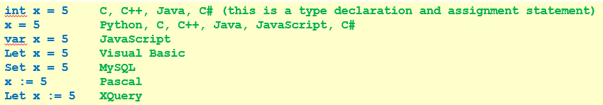
An assignment statement is a fundamental part of every computer program. It is a computer operation that stores a value in a memory location identified by a [named] variable. The following example shows assignment statements from other programming languages:
In R, there are three ways to perform an assignment statement:
|
x <- 5
x
[1] 5
|
x = 5
x
[1] 5
|
5 -> x
x
[1] 5
|
They all say: assign 5 to x, store 5 at x, or set x to 5. This instruction will use the middle way (most of the time)!
Simple R Variables, Objects, and Data Types
character (e.g. 'Mike')
real (floating point, double) numbers (e.g. 0.05)
integer (e.g. 30)
complex (e.g. 1 + 2i)
logical (e.g. FALSE, TRUE)
Important note:
As opposed to other programming languages, R does not have scalar types. Even if a variable is assigned a single value, the variable is treated as a vector (the simplest R data structure). As single-valued variables,
they do not have to use an index which is mandatory for multi-valued data structures.
You can examine the type of the variable using functions class() and typeof().
Numeric Variables (double)
There in no declaration of the type for R variables. The variables adopt their type from the values or expressions they are assigned to. In the following example, value 5 is a numeric value. The smallest positive value of the double type is 2.225074e-308; the largest one—1.797693e+308.
x = 5
x
[1] 5
class(x)
[1] "numeric"
typeof(x)
[1] "double"
Notice an index [1] notation shown in front of the variable value. R is telling as that it is a vector. With a signgle-valued variable x is the same as x[1].
The following examples show a variable (y) being set to an expression (x + 1).
It inherits the type from the expression in which both the components are of numeric (double) type:
y = x + 1
y
[1] 6
class(y)
[1] "numeric"
typeof(y)
[1] "double"
Numeric Variables (integer)
A single-valued, integer variable:
n = 10L
n
1] 5
class(n)
[1] "integer"
typeof(n)
[1] "integer"
As you can see, in order to force a single value to be an integer, we add letter L to the number.
In the following example, variable m is set to a sequence of whole numbers (1,2,…,8):
m = 4:8
m
[1] 4 5 6 7 8
class(m)
[1] "integer"
typeof(m)
[1] "integer"
m[2]
[1] 5
m[2:4]
[1] 5 6 7
Notice the way vector m values can be accessed via its index. Notation [2:4] gets the sequence (sub-vectors) at consecutive index positions 2 through 4.
Numeric Variables (complex)
Complex numbers have serious applications in Math and Physics, particularly in Electronics and Electromagnetism. They are shown here for completeness.
c = 3 + 2i
c
[1] 3+2i
class(c)
[1] "complex"
typeof(c)
[1] "complex"
c = complex(real = 3, imaginary = 2)
c
[1] 3+2i
Also try this:
d = sqrt(-1)
d
[1] NaN # Not a Number
d = sqrt(as.complex(-1))
d
[1] 0+1i
Character (String) Variables
Consider the following example
first_name = 'Ann'
first_name
[1] "Ann"
first_name[1]
1] "Ann"
class(first_name)
[1] "character"
Contrary to many other programming languages, the entire string is stored at the index position 1.
To access individual characters function
substr() can be used. For example:
full_name = 'Ann J Fortran'
full_name
[1] "Ann J Fortran"
first_name = substr(full_name,1,3)
first_name
[1] "Ann"
last_name = substr(full_name,7,13)
last_name
[1] "Fortran"
middle_initial = substr(full_name,5,5)
middle_initial
[1] "J"
Function substr() uses three arguments (string, from_position, to_position).
A logical variable can represent one of the two states: TRUE or FALSE.
is_young = TRUE
is_young
[1] TRUE
ann_age = 25
tom_age = 30
ann_is_younger = ann_age < tom_age
ann_is_younger
[1] TRUE
tom_is_younger = tom_age < ann_age
tom_is_younger
[1] FALSE
ann_is_younger = !tom_is_younger
ann_is_younger
[1] TRUE
Notice the exclamation point (!) working as negation operator (not FALSE is TRUE).
Arithmetical operators are used in numeric expressions.
Operator | Meaning | Example | Result
|
+ | Addition | 2+5 | 7
|
- | Subtraction | 43650 | 3
|
* | Multiplication | 3*8 | 24
|
/ | Division | 43803 | 3
|
%/% | Integer Division | 9%/%4 | 2
|
%% | Division Remainder | 9%%4 | 1
|
^ or ** | Exponentiation | 3^4 | 81
|
Relational operators are use to build relational (comparison) expressions.
Operator | Meaning | Example | Result
|
< | Less Than | 2 < 5 | TRUE
|
<= | Less Than or Equal To | 4 <= 4 | TRUE
|
== | Equal To | 3 == 9/3 | TRUE
|
> | Greater Than | 2 > 5 | FALSE
|
>= | Greater Than or Equal To | 4 >= 4 | TRUE
|
!= | Not Equal To | 2 != 2 | FALSE
|
Logical operator are used to construct logical (TRUE/FALSE) expressions.
Operator | Meaning | Example | Result
|
! | Negation (NOT) | !TRUE | FALSE
|
& | Intersection (AND) | TRUE & FALSE | FALSE
|
| | Alternative (OR) | TRUE | FALSE | TRUE
|
Structured R Variables, Objects, and Data Types
vector - a sequence of data of the same type, e.g. c(2,5,1,7,4)
lista list of data of possibly different types, e.g. list(1,"A",c(4,8,5))
arraya multidimensional array, array(c(1,2,3,4,5,6,7,8),dim = c(2,2,2))
matrix – a two-dimensional array, e.g. matrix(c(1,2,3,4,5,6), nrow=2, ncol=3, byrow=TRUE)
dataframe – a table (e.g. mtcars)
Vectors are ordered collections of objects (elements or components) of the same type.
A sequence of natural numbers (1,2,...,8).
v = 1:8
v
[1] 1 2 3 4 5 6 7 8
typeof(v)
[1] "integer"
Function seq.int() generates a sequence of numbers from first to not less than last, advanced by increment.
v1 = seq.int(1L,5L,2L)
v1
[1] 1 3 5
v2 = seq.int(2L,6L,2L)
v2
[1] 2 4 6
Operators used with vectors perform the operations on all vector elements:
v
[1] 1 2 3 4 5 6 7 8
sqr_v = v ^ 2
sqr_v
[1] 1 4 9 16 25 36 49 64
Vectors of Doubles [Double Precision Numbers]
A sequence of real numbers (1.0,2.5,2,2.5,...,8.5,9.0).
v = seq.int(1,9,0.5)
v
[1] 1.0 1.5 2.0 2.5 3.0 3.5 4.0 4.5 5.0 5.5 6.0 6.5 7.0 7.5 8.0 8.5 9.0
n = length(v)
n
[1] 17
Write an expression to return the difference between consecutive numbers of the vector v.
(Second – First, Third – Second, Fourth – Third, . . ., Last – Second Last.)
v[2:n]-v[1:n-1]
[1] 0.5 0.5 0.5 0.5 0.5 0.5 0.5 0.5 0.5 0.5 0.5 0.5 0.5 0.5 0.5 0.5
The differences are fixed as the vector, v,has been created as a sequence with a fixed increment (here 0.5).
Add them up:
v_sum = sum(v)
v_sum
[1] 85
Generate a more descriptive output, using the cat() function.
cat('The sum of \n '); cat(v); cat('\nis: '); cat(v_sum); cat('\n');
The sum of
1 1.5 2 2.5 3 3.5 4 4.5 5 5.5 6 6.5 7 7.5 8 8.5 9
is: 85
Using the c() function. Think of it as "combine elements" or "concatenate elements" into a vector.
vec = c(3,5,7,8,9)
vec
[1] 3 5 7 8 9
n = length(vec)
n
[1] 5
sum(vec)/length(vec)
[1] 6.4
Same as:
mean(vec)
[1] 6.4
R coerces vector elements into the most "agreeable" type.
Create a vector of integers:
ints = c(1:5)
ints
[1] 1 2 3 4 5
typeof(ints)
[1] "integer"
Create a vector of doubles (made of explicit integers (1:5) and one implicit double (6):
dbls = c(1:5,6)
dbls
[1] 1 2 3 4 5 6
typeof(dbls)
[1] "double"
Such data type conversion is based on the principle of data integrity that prevents loss of data (or precision).
Moving from "integer" to "double" is generally safe but not the other way around.
In many situations we may need to initialize vectors. The following examples show two applications of the rep() function that creates vectors by replicating numbers or other vectors.
vect1 = rep(0,5)
vect1
[1] 0 0 0 0 0
vect2 = rep(c(1,2,3),5)
vect2
[1] 1 2 3 1 2 3 1 2 3 1 2 3 1 2 3
Use the append() function to append new data to the end of a vector or to insert the data at some inner position. Let's first append new content at the end of vector vect1.
vect1 = append(vect1,rep(1,5))
vect1
[1] 0 0 0 0 0 1 1 1 1 1
Next, insert number 2 before position 1 in vector vect1.
vect1 = append(vect1,2,0)
vect1
[1] 2 0 0 0 0 0 1 1 1 1 1
Vectors of Logical Values
Logical vectors combine logical values FALSE, TRUE.
Let's replicate FALSE seven times.
bool_vec = rep(FALSE, 7)
bool_vec
[1] FALSE FALSE FALSE FALSE FALSE FALSE FALSE
Here is another way of doing it:
bool_vec = vector("logical", 7)
bool_vec
[1] FALSE FALSE FALSE FALSE FALSE FALSE FALSE
Logical values are usually produced by logical expression. The following example shows outcomes for three logical (relational) expressions that are stored in a logical vector, vbool.
x = 5
vbool = c(x < 5, x == 5, x > 5)
vbool
[1] FALSE TRUE FALSE
Let's create a vector of names and then sort the vector alphabetically.
fn = c('Ken','Ann','Tom','Eve','Pat','Don','Kim','Sue')
fn
[1] "Ken" "Ann" "Tom" "Eve" "Pat" "Don" "Kim" "Sue"
sorted_fn = sort(fn)
sorted_fn
[1] "Ann" "Don" "Eve" "Ken" "Kim" "Pat" "Sue" "Tom"
What about a descending order?
sorted_desc_fn = sort(fn, decreasing = FALSE)
sorted_desc_fn
[1] "Tom" "Sue" "Pat" "Kim" "Ken" "Eve" "Don" "Ann"
Get lengths of all strings stored in a vector.
fnm = c('Kim','Debb','Chris','Jeanny','Michael')
str_lengths = nchar(fnm)
str_lengths
[1] 3 4 5 6 7
Vectors with Named Elements
Typically, we access data elements from vectors by index. For example:
age = c(22,29,35,50,65)
age
[1] 22 29 35 50 65
Show second, third and last elements:
age(c(2,3,5))
[1] 29 35 65
Let's name and access vector elements by name.
names(age) = c('Dan','Eve','Fox','Jan','Kam')
age
Dan Eve Fox Jan Kam
22 29 35 50 65
age['Kam']
Kam
65
age['Eve']
Eve
29
age[c('Dan','Jan')]
Dan Jan
22 50
With named elements, vectors can be used as dictionaries (lookup sources).
A list may contain objects of different sizes.
List of String Groups (Vectors)
Create a list element contains vectors of strings of different sizes.
grp1 = c('Ken','Ann','Tom')
grp2 = c('Eve','Pat')
grp3 = c('Don','Kim','Sue','Ron')
grps = list(grp1,grp2,grp3)
grps
[[1]]
[1] "Ken" "Ann" "Tom"
[[2]]
[1] "Eve" "Pat"
[[3]]
[1] "Don" "Kim" "Sue" "Ron"
Let's find out more about this list.
Get the first list's member:
grps[[1]]
[1] "Ken" "Ann" "Tom"
Get the second name of the 3rd list's member.
Find out the size of the list.
Get the length of the 1st member (vector).
Get the length of the 2nd member (vector).
Get the length of the 3rd member (vector).
List of Strings and Integers
A list may contain objects of different types. Here, each list element contains vectors of different types.
name = c('Ken', 'Ann', 'Tom')
age = c(25, 19, 33)
people = list(name, age)
people
[[1]]
[1] "Ken" "Ann" "Tom"
[[2]]
[1] 25 19 33
Let's write a statement about Ken's age, using function cat().
cat(people[[1]][1]); cat(' is '); cat(people[[2]][1]); cat(' years old.'); cat('\n')
Ken is 25 years old.
Function cat() is used to print a single object. Statement cat('\n') performs a line feed (same as the Enter key does).
Notice that this program line contains multiple statements. Typically, we write each statement on a separate line. R statements that
appear on the one line must be separated with a colon (;).
A list may have named elements. Thus it can work as a dictionary, a key-value structure.
Let's redefine the people list. This time, we will store the names as keys.
people = list(Ken=25,Ann=19, Tom=33)
people
$Ken
[1] 25
$Ann
[1] 19
$Tom
[1] 33
How old is Ann?
cat('Ann'); cat(' is '); cat(people$Ann); cat(' years old.'); cat('\n')
Ann is 19 years old.
Notation people$Ann is equivalent to people[[2]][1].
cat('Ann'); cat(' is '); cat(people[[2]][1]); cat(' years old.'); cat('\n')
Ann is 19 years old.
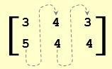
An array is a multi-dimensional structure, in which each dimension holds the same number of elements. In a two-dimensional array, each row has the same length and each column has the same length. Because of these properties, arrays are also referred to a rectangular structures. Again, a two-dimensional array looks like a rectangle. Here is an example of a two-dimensional array (2 by 3):
x = array( c(3,5,4,4,3,4), dim=c(2,3) )
x
| | [,1] | [,2] | [,3] |
| [1,] | 3 | 4 | 3 |
| [2,] | 5 | 4 | 4 |
This array is arranged by columns. The first two values are placed in the first column, the second two values—in the second column, etc.
Array dimensions can also be named.
dn = list( c('r1','r2'), c('c1','c2','c3') )
y = array( c(3,5,4,4,3,4), dim=c(2,3), dimnames=dn )
y
Accessing arrays by index.
x = array( c(3,5,4,4,3,4), dim=c(2,3) )
x
| | [,1] | [,2] | [,3] |
| [1,] | 3 | 4 | 3 |
| [2,] | 5 | 4 | 4 |
Get the element from the 2nd row and 1st column.
Get the elements from the 2nd column (all rows intersecting this column).
Get the elements from the 2nd row (all columns intersecting this row).
Get the elements from columns 2 and 3 (all rows intersecting these columns).
Accessing arrays by name.
y
y['r1',]
c1 c2 c3
3 4 3
y[,'c2']
r1 r2
4 4
y['r2','c3']
[1] 4
A matrix is a two dimensional array. As numeric arrays, matrices are very convenient and vary powerful data containers in Data Science.
They are based on the concept of matrices as defined in Linear Algebra. Here is an m x n matrix named as A,
having m rows and n columns.
| A = |
| a11 | a12 | … | a1j | … | a1n |
| a21 | a22 | … | a2j | … | a2n |
| ⋮ | ⋮ | … | ⋮ | … | ⋮ |
| ai1 | ai2 | … | aij | … | ain |
| ⋮ | ⋮ | … | ⋮ | … | ⋮ |
| am1 | am2 | … | amj | … | amn |
|
A matrix, S, having the same number of rows (m) and columns (m) is referred to as a Square matrix.
| S = |
| a11 | a12 | … | a1i | … | a1m |
| a21 | a22 | … | a2i | … | a2m |
| ⋮ | ⋮ | … | ⋮ | … | ⋮ |
| ai1 | ai2 | … | aii | … | aim |
| ⋮ | ⋮ | … | ⋮ | … | ⋮ |
| am1 | am2 | … | ami | … | amm |
|
A square matrix, D, with all zeros except for the left-down diagonal is called a Diagonal matrix.
| D = |
| a11 | 0 | … | 0 | … | 0 |
| 0 | a22 | … | 0 | … | 0 |
| ⋮ | ⋮ | … | ⋮ | … | ⋮ |
| 0 | 0 | … |
aii |
… | 0 |
| ⋮ | ⋮ | … | ⋮ | … | ⋮ |
| 0 | 0 | … | 0 | … |
amm |
|
A Diagonal matrix, I, with all diagonal values of 1 is referred to as an Identity matrix.
| I = |
| 1 | 0 | … | 0 | … | 0 |
| 0 | 1 | … | 0 | … | 0 |
| ⋮ | ⋮ | … | ⋮ | … | ⋮ |
| 0 | 0 | … | 1 | … | 0 |
| ⋮ | ⋮ | … | ⋮ | … | ⋮ |
| 0 | 0 | … | 0 | … | 1 |
|
Creating a matrix from a vector.
mx = matrix( c(3,5,4,4,3,4), nrow = 2, ncol = 3 )
mx
| | [,1] | [,2] | [,3] |
| [1,] | 3 | 4 | 3 |
| [2,] | 5 | 4 | 4 |
|
Matrix mx is arranged by columns (by default). The first two values of the vector argument, c(3,5,4,4,3,4), are placed in the first column,
the second two values—in the second column, etc. |
 |
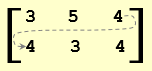
Try this to arrange data by rows:
my = matrix( c(3,5,4,4,3,4), nrow = 2, ncol = 3, byrow=TRUE )
my
| | [,1] | [,2] | [,3] |
| [1,] | 3 | 5 | 4 |
| [2,] | 4 | 3 | 4 |
|
Matrix my is arranged by columns. The first three values are placed in the first row, the second three values—in the second row.
|
|
Matrices can be manipulated mathematically (like in Linear Algebra).
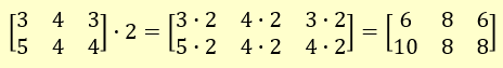
Multiply a matrix by a number:
mx = matrix( c(3,5,4,4,3,4), nrow = 2, ncol = 3 )
mx
| | [,1] | [,2] | [,3] |
| [1,] | 3 | 4 | 3 |
| [2,] | 5 | 4 | 4 |
m1x = mx * 2
m1x
| | [,1] | [,2] | [,3] |
| [1,] | 6 | 8 | 6 |
| [2,] | 10 | 8 | 8 |
Each of the matrix elements is multiplied by the number (here 2).
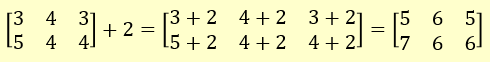
Add a number to a matrix:
mx = matrix( c(3,5,4,4,3,4), nrow = 2, ncol = 3 )
mx
| | [,1] | [,2] | [,3] |
| [1,] | 3 | 4 | 3 |
| [2,] | 5 | 4 | 4 |
m2x = mx + 2
m2x
| | [,1] | [,2] | [,3] |
| [1,] | 5 | 6 | 5 |
| [2,] | 7 | 6 | 6 |
Number 2 is added to each element of the matrix.
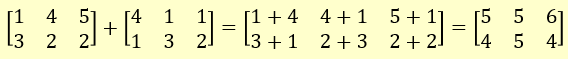
Add two matrices:
|
dat1 = c(1,3,4,2,5,2)
mx1 = matrix( dat1, nrow = 2, ncol = 3 )
mx1
| | [,1] | [,2] | [,3] |
| [1,] | 1 | 4 | 5 |
| [2,] | 3 | 2 | 2 |
|
dat2 = c(4,1,1,3,1,2)
mx2 = matrix( dat2, nrow = 2, ncol = 3 )
mx2
| | [,1] | [,2] | [,3] |
| [1,] | 4 | 1 | 1 |
| [2,] | 1 | 3 | 2 |
|
|
mx3 = mx1 + mx2
mx3
| | [,1] | [,2] | [,3] |
| [1,] | 5 | 5 | 6 |
| [2,] | 4 | 5 | 4 |
|
The matrices are added by elements.
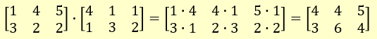
Multiply two matrices by elements (an element-wise matrix multiplication):
|
dat1 = c(1,3,4,2,5,2)
mx1 = matrix( dat1, nrow = 2, ncol = 3 )
mx1
| | [,1] | [,2] | [,3] |
| [1,] | 1 | 4 | 5 |
| [2,] | 3 | 2 | 2 |
|
dat2 = c(4,1,1,3,1,2)
mx2 = matrix( dat2, nrow = 2, ncol = 3 )
mx2
| | [,1] | [,2] | [,3] |
| [1,] | 4 | 1 | 1 |
| [2,] | 1 | 3 | 2 |
|
|
mx3 = mx1 * mx2
mx3
| | [,1] | [,2] | [,3] |
| [1,] | 4 | 4 | 5 |
| [2,] | 3 | 6 | 4 |
|
This type of matrix multiplication is a vector driven (element wise) multiplication. The matrices must be of the same size.
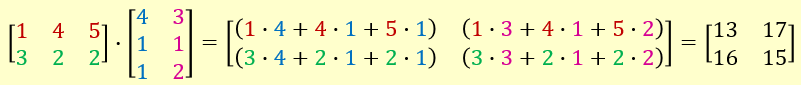
Multiply two matrices as in Linear Algebra (a pure matrix multiplication):
|
dat1 = c(1,3,4,2,5,2)
mx1 = matrix( dat1, nrow = 2, ncol = 3 )
mx1
| | [,1] | [,2] | [,3] |
| [1,] | 1 | 4 | 5 |
| [2,] | 3 | 2 | 2 |
|
dat2 = c(4,1,1,3,1,2)
mx2 = matrix( dat2, nrow = 3, ncol = 2 )
mx2
| [,1] | [,2] |
| [1,] | 4 |
3 |
| [2,] |
1 |
1 |
| [3,] | 1 |
2 |
|
|
mx3 = mx1 %*% mx2
mx3
| | [,1] | [,2] |
| [1,] | 13 | 17 |
| [2,] | 16 | 15 |
|
The two matrices must be conformable, that is the number of columns in the first matrix must be equal to the number of rows in the second matrix.
This operation is performed in Excel by function MMULT().
The elements of the resulting matrix are cross-products of rows in the first matrix and columns in the second matrix.
A cross product of two equally sized vectors is the sum of the product of the elements of the vectors at the same position.
Such and operation is done in Excel, using the SumProduct() function. For two vectors, v1 and v2, R can calculate the cross-product as crossprod(v1,v2) or as v1 %*% v2. In either case the outcome is a matrix. To produce a [plain] number, force the outcome to be a number: as.numeric(crossprod(v1,v2)) and as.numeric(v1 %*% v2).
Calculate an inverse matrix.
vx = c(2,1,4,3,2,1,1,3,3)
mx = matrix( vx, nrow = 3, ncol = 3 )
mx
| [,1] | [,2] | [,3] |
| [1,] | 2 | 3 | 1 |
| [2,] 1 2 3 | 1 | 2 | 3 |
| [3,] 4 1 3 | 4 | 1 | 3 |
In Linear Algebra, if A is a square matrix then its inverse is denoted by A-1. R gets the inverse matrix, using the solve() function::
inv_mx = solve(mx)
inv_mx
| [,1] | [,2] | [,3] |
| [1,] | 0.1153846 | -0.30769231 | 0.26923077 |
| [2,] 1 2 3 | 0.3461538 | 0.07692308 | -0.19230769 |
| [3,] 4 1 3 | -0.2692308 | 0.38461538 | 0.03846154 |
This operation is performed in Excel by function MINVERSE().
The input matrix must be square. An inverse matrix multiplied by the original matrix will produce an Identity matrix:
mx %*% inv_mx
| [,1] | [,2] | [,3] |
| [1,] | 1 | 0 | -7.632783E-17 |
| [2,] 1 2 3 | -1.110223E-16 | 1 | 0 |
| [3,] 4 1 3 | 0 | 0 | 1 |
Due to rounding imprecision, the above output does not look like a perfect Identity matrix. Here is a rounded result (rounded to 12 decimal digits after the decimal period:
round(mx %*% inv_mx,12)
| [,1] | [,2] | [,3] |
| [1,] | 1 | 0 | 0 |
| [2,] 1 2 3 | 0 | 1 | 0 |
| [3,] 4 1 3 | 0 | 0 | 1 |
Solving a Linear Equation System
In general, using a matrix notation, a linear equation system and its solution can be expressed as follows:
For the following equation system:
2x1 + 3x2 + 1x3 = 630
1x1 + 2x2 + 3x3 = 550
4x1 + 1x2 + 3x3 = 600
matrix A is defined by the coefficients of the [unknown] variables:
2 3 1
1 2 3
4 1 3
In R:
v = c(2,3,1,1,2,3,4,1,3)
A = matrix( v, nrow = 3, ncol = 3, byrow=T)
A
| [,1] | [,2] | [,3] |
| [1,] | 2 |
3 |
1 |
| [2,] |
1 | 2 |
3 |
| [3,] |
4 |
1 | 3 |
Vector b represents the right-hand side values:
630
550
600
In R:
b = c(630,550,600)
b
[1] 630 550 600
The solution (here x1, x2, x3) is provided as a matrix product of the inverse matrix and the right-hand side vector.
x = solve(A) %*% b
x
| | [,1] |
| [1,] | 65 |
| [2,] | 145 |
| [3,] | 65 |
Solution: x1 = 65, x2 = 145, x3 = 65. As a check, if you multiply matrix A by vector x (A∙x), you should get the right-hand side vector:
A %*% x
| | [,1] |
| [1,] | 630 |
| [2,] | 550 |
| [3,] | 600 |
Special matrix cases.
Diagonal:
diag(c(4,6,7))
| [,1] | [,2] | [,3] |
| [1,] | 4 | 0 | 0 |
| [2,] | 0 | 6 | 0 |
| [3,] | 0 | 0 | 7 |
Identity:
diag(3)
| [,1] | [,2] | [,3] |
| [1,] | 1 | 0 | 0 |
| [2,] | 0 | 1 | 0 |
| [3,] | 0 | 0 | 1 |
Matrix x transposed (xT):
Transpose (xT):
Matrix Operations on Vectors!
Consider two vectors, v1 and v2.
v1 = c(4,6,2,1)
v1
[1] 4 6 2 1
v2 = c(1,2,1,1)
v2
[1] 1 2 1 1
Now, calculate a sum of the products of the vector elements (the same as =SumProduct() in Excel).
Note: In this case, it may be safer to use the crossprod() function:
Multiply the vectors as matrices (the same as =MMult() in Excel). The second vector must be transposed. Otherwise the matrices (based on the vectors) would not be conformable.
v1 %*% t(v2)
| | [,1] | [,2] | [,3] | [,4] |
| [1,] | 4 | 8 | 4 | 4 |
| [2,] | 6 | 12 | 6 | 6 |
| [3,] | 2 | 4 | 2 | 2 |
| [4,] | 1 | 2 | 1 | 1 |
Note: this matrix is a collection of the products of all possible pairings of the vector values.
| 1 | 2 | 1 | 1 | |
| 4*1 | 4*2 | 4*1 | 4*1 | 4 |
| 6*1 | 6*2 | 6*1 | 6*1 | 6 |
| 2*1 | 2*2 | 2*1 | 2*1 | 2 |
| 1*1 | 1*2 | 1*1 | 1*1 | 1 |
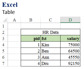
Data frames are table-like structures (similar to Excel tables). They are extremely popular among data analysts.
If you have worked with spreadsheet tables, you will find R data frames also friendly but also very powerful.
 |
 |
| Data Access: |
| pid: | B4:B7 |
| fst: | C4:C7 |
| salary: | D4:D7 |
| row 1: | B4:D4 |
| row 3: | B6:D6 |
|
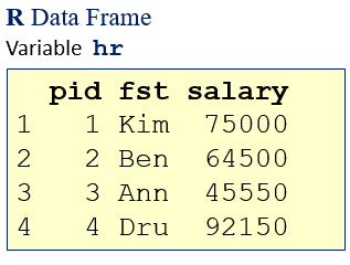
| Data Access: |
| pid: | hr$pid / hr[,1] / hr[[1]] / hr[1] |
| fst: | hr$fst / hr[,2] / hr[[2]] / hr[2] |
| salary: | hr$salary / hr[,3] / hr[[3]] / hr[3] |
| row 1: | hr[1,] |
| row 3: | hr[3,] |
|
| It is also possible to assign names to the ranges.
|
Notice that notation hr[1] gets the entire
column 1 as a data frame. |
Create a data frame (df_hr), consisting of three columns: person ID, person_id, first name, first_name,
and annual salary, annual_salary. One way to create a data frame is to assemble it, using columns defined separately as vectors.
person_id = c(1:4)
first_name = c("Kim","Ben","Ann","Dru")
annual_salary = c(75000,64500,45550,92150)
df_hr = data.frame( person_id, first_name, annual_salary)
df_hr
  person_id first_name annual_salary
1         1        Kim         75000
2         2        Ben         64500
3         3        Ann         45550
4         4        Dru         92150
R has done a few interesting things. It used the names of the [input] vectors as the data frame's column names. This can be changed by giving the names explicitly (e.g. as pid, fst, and salary):
hr = data.frame( pid=person_id, fst=first_name, salary=annual_salary)
hr
  pid fst salary
1   1 Kim  75000
2   2 Ben  64500
3   3 Ann  45550
4   4 Dru  92150
Let's try a few ways to access data from data frame hr.
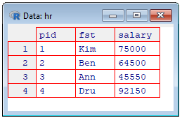
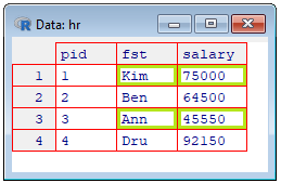
Show the data frame in a grid (spreadsheet):
View(hr)
Show all data in column 1 as a data frame:
Show all data in row 2 (all columns) as a data frame:
hr[2,]
  pid fst salary
2   2 Ben  64500
Show all data in column 1 (all rows) as a vector:
hr[[1]] # same as hr$pid or hr[,1]
[1] 1 2 3 4
Show all data in row 2 (all columns) as [flat] vector:
as.character(hr[2,])
[1] "2" "2" "64500"
Let's try a few more ways to access data from data frame hr.
|
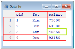
Show the salary value for Ann:
hr[hr$fst=='Ann',3] # same as hr[hr$fst=='Ann',]$salary
[1] 45550
|
|
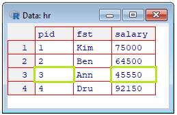
Show the person ID and salary value for Ann:
hr[hr$fst=='Ann',c(1,3)]
pid salary
3 3 45550
|
Print the person ID and salary value for Ann, using the cat() function:
cat(hr[hr$fst=='Ann',c(1,3)])
Error in cat(hr[hr$fst == "Ann", c(1, 3)]) :
argument 1 (type 'list') cannot be handled by 'cat'
Try this way:
cat(unlist(hr[hr$fst=='Ann',c(1,3)]))
3 45550
|
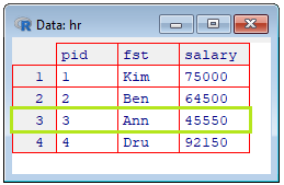
Show the Ann's salary record:
ann_record = hr[hr$fst=='Ann',]
ann_record
pid fst salary
3 3 Ann 45550
|
We know that variable ann_record can't be printed by the cat() function, unless the variable is flattened (unlisted). Let’s see what happened when we do it:
ar = unlist(ann_record)
cat(ar)
3 1 45550
We got an interesting output: pid = 3, fst = 1, and salary = 45550. It all looks reasonable (?) except for fst.
It is supposed to be equal to 'Ann' but it shows 1. Well, if we examine column fst, we will see that it does not show quoted strings.
It also shows the so called levels.
hr$fst
[1] Kim Ben Ann Dru
Levels: Ann Ben Dru Kim
During construction of the frame, R has converted the string vector, first_name, to a factor vector.
All the string data got mapped to integers for faster processing. See the examples for more details.
Let's find out more about the factors assigned to fst strings.
Show column fst as a numeric vector:
fst_fct = as.numeric(hr$fst)
fst_fct
[1] 4 2 1 3
In a database world, we would say that R indexed the names. Notice that the factor values are assigned to the strings
according to the alphabetical order. Kim → 4, Ben → 2, Ann → 1, Dru →3. It is much easier to process ordered data than—random data. It is particularly advantageous when processing large data sets. It is possible (but not advisable) to convert the column to character (string) data.
hr$fst = as.character(hr$fst)
hr$fst
[1] "Kim" "Ben" "Ann" "Dru"
When displaying the entire data frame, hr, the quotes are not shown.
hr
  pid fst salary
1   1 Kim  75000
2   2 Ben  64500
3   3 Ann  45550
4   4 Dru  92150
As shown above, data frames can be queried. Rows, columns, and their fragments can be filtered out.
Let's try to build a filter that will allow us to select specific rows.
m = nrow(hr)
filter = rep(TRUE, m)
filter
[1] TRUE TRUE TRUE TRUE
hr[filter,]
  pid fst salary
1   1 Kim  75000
2   2 Ben  64500
3   3 Ann  45550
4   4 Dru  92150
Since all the values of variable filter, placed at the row reference, are TRUE, all the rows are displayed. Let's modify the filter,
by setting the 2nd and 4th values to FALSE and then repeat the same statement.
filter[c(2,4)] = FALSE
filter
[1] TRUE FALSE TRUE FALSE
hr[filter,]
  pid fst salary
1   1 Kim  75000
3   3 Ann  45550
There are many ways to create filters. Let's try a few more examples. First, show records, with salaries below 70,000.
filter = hr$salary < 70000
filter
[1] FALSE TRUE TRUE FALSE
hr[filter,]
  pid fst salary
2   2 Ben  64500
3   3 Ann  45550
What about salaries between 60,000 and 80,000?
filter = hr$salary >= 60000 & hr$salary <= 80000
filter
[1] TRUE TRUE FALSE FALSE
hr[filter,]
  pid fst salary
1   1 Kim  75000
2   2 Ben  64500
Note: The sqldf library provides powerful functions to query data frames, using SQL.
Let’s get the salaries above the average.
avg_salary = mean(hr$salary)
avg_salary
[1] 69300
filter = hr$salary > avg_salary
filter
hr[filter,]
  pid fst salary
1   1 Kim  75000
4   4 Dru  92150
|
Finally, let’s show data at the intersection of rows 1, 4 and columns 2, 3.
hr[c(1,4),c(2,3)]
  fst salary
1 Kim  75000
4 Dru  92150
|
There are other ways to create data frames. Suppose that we need to gradually add rows to a data frame. We start with an empty frame and we add rows in a loop. The following investment example illustrated this concept. We invest an initial value (e.g. principal = $1,000) at the begining of the first year. At the end of the year we add interest to the investemnt (based on rate = 5%) which gets reinvested at the beginign of the next year. We repeat this procedure for 10 years (term = 10).
principal = 1000
rate = 0.05
term = 10
# Create an empty frame with three columns of type: integer, double, double.
cash_earned = data.frame(year=integer(0), beginning=double(0), ending=double(0))
investment = principal
for (y in 1:term) {
beg = investment
investment = (1 + rate) * investment
# Create a one-row frame with values for columns: year, beginning, ending.
new_cash = data.frame(year=y, beginning=beg, ending=investment)
# Bind the original data frame with the new one (by rows).
cash_earned = rbind(cash_earned, new_cash)
}
cash_earned
     year beginning   ending
1     1  1000.000 1050.000
2     2  1050.000 1102.500
3     3  1102.500 1157.625
4     4  1157.625 1215.506
5     5  1215.506 1276.282
6     6  1276.282 1340.096
7     7  1340.096 1407.100
8     8  1407.100 1477.455
9     9  1477.455 1551.328
10   10  1551.328 1628.895
Data
R comes not only with programming capabilities. The R installer also add some data to the R environment.
Let's try a built-in dataframe mtcars.
cars = mtcars
head(cars)
                   mpg cyl disp  hp drat    wt  qsec vs am gear carb
Mazda RX4         21.0   6  160 110 3.90 2.620 16.46  0  1    4    4
Mazda RX4 Wag     21.0   6  160 110 3.90 2.875 17.02  0  1    4    4
Datsun 710        22.8   4  108  93 3.85 2.320 18.61  1  1    4    1
Hornet 4 Drive    21.4   6  258 110 3.08 3.215 19.44  1  0    3    1
Hornet Sportabout 18.7   8  360 175 3.15 3.440 17.02  0  0    3    2
Valiant           18.1   6  225 105 2.76 3.460 20.22  1  0    3    1
attributes(cars)
$names
 [1] "mpg"  "cyl"  "disp" "hp"   "drat" "wt"   "qsec" "vs"   "am"   "gear" "carb"
$row.names
 [1] "Mazda RX4"           "Mazda RX4 Wag"       "Datsun 710"          "Hornet 4 Drive"      "Hornet Sportabout"   "Valiant"
 [7] "Duster 360"          "Merc 240D"           "Merc 230"            "Merc 280"            "Merc 280C"           "Merc 450SE"
[13] "Merc 450SL"          "Merc 450SLC"         "Cadillac Fleetwood"  "Lincoln Continental" "Chrysler Imperial"   "Fiat 128"
[19] "Honda Civic"         "Toyota Corolla"      "Toyota Corona"       "Dodge Challenger"    "AMC Javelin"         "Camaro Z28"
[25] "Pontiac Firebird"    "Fiat X1-9"           "Porsche 914-2"       "Lotus Europa"        "Ford Pantera L"      "Ferrari Dino"
[31] "Maserati Bora"       "Volvo 142E"
$class
[1] "data.frame"
R can also parse text and load it into a dataframe.
hr = read.table(text='
pid fst salary
1 Kim 75000
2 Ben 64500
3 Ann 45550
4 Dru 92150'
, header = TRUE)
hr
  pid fst salary
1   1 Kim  75000
2   2 Ben  64500
3   3 Ann  45550
4   4 Dru  92150
Many data science project with R are done, using data that come from external sources (local file, Web document, database, etc.).
R is equipped with many functions that can retrieve data (usually into data frames) from such resources.
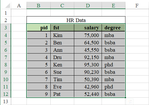
A popular way is to transfer data via the system's Clipboard. Here is how to copy data from a spreadsheet (Excel) document.
Step 1. Launch R.
Step 2. (prepare an R statement to receive data). Do not press Enter at the end of the statement's line.
x = read.table(file="clipboard", sep ="\t", header=TRUE)
Step 3. Open the
Excel's dataset (workbook). Try this workbook
hr.xlsx.
Step 4. Select the table you want to send to R, (in hr.xlsx, select range B3:E12)
and press the Copy button (or hit keys Ctrl+C).
Step 5. Switch back to R and press the Enter key (while the cursor is still flashing at the end of the above statement).
If the statement has been entered prior to copying the dataset in Excel, just press the UP Arrow key
(to recall the statement) and then press Enter.
Show the table.
x
  pid   fst   salary degree
1   1  Kim   75,000    mba
2   2  Ben   64,500   bsba
3   3  Ann   45,550   bsba
4   4  Dru   92,150    mba
5   5  Ken   95,300    phd
6   6  Sue   90,230   bsba
7   7  Tim   50,390    mba
8   8  Eve   42,960    phd
9   9  Pat   52,440   bsba
Get Data From a Web Document
It is very easy to load data into R from Web files. Most frequently such data sources are stored as the so called Comma Separated Values (CSV).
Excel refers to such file types as CSV (Comma delimited) (*.csv). To save an Excel worksheet as a CSV file, use the File > Save As command and
change the file type to CSV (Comma delimited) (*.csv) via the Save as type: drop-down option.
The following example shows how to load data from URL
hr.csv.
x = read.csv('http://biiat.com/dat/hr.csv', header=TRUE)
x
              pid   fst   salary degree
1   1  Kim   75,000    mba
2   2  Ben   64,500   bsba
3   3  Ann   45,550   bsba
4   4  Dru   92,150    mba
5   5  Ken   95,300    phd
6   6  Sue   90,230   bsba
7   7  Tim   50,390    mba
8   8  Eve   42,960    phd
9   9  Pat   52,440   bsba
Get Data From a Local Document
Another popular data source is a local text document. The procedure for loading data from a local file to a data frame is very similar to
the previous one (shown on the previous slide). All it takes is replacing the Web address with local file reference.
For example, file hr.csv, residing in folder T:\rdev, would be retrieved into a data frame in the following way:
x = read.csv('T:/rdev/hr.csv', header=TRUE)
x
  pid   fst   salary degree
1   1  Kim   75,000    mba
2   2  Ben   64,500   bsba
3   3  Ann   45,550   bsba
4   4  Dru   92,150    mba
5   5  Ken   95,300    phd
6   6  Sue   90,230   bsba
7   7  Tim   50,390    mba
8   8  Eve   42,960    phd
9   9  Pat   52,440   bsba
What about getting a simple sample from a [plain] text document to a vector (
txt)?
Let’s first download file
names.txt from
names into folder
T:/rdev/. Next read the file, using function
scan().
txt = scan('T:/rdev/names.txt', character())
Read 483 items
txt[1:50] # Show the firsts 50 values.
[1] "Kim" "Dan" "Pat" "Pat" "Pat" "Kim" "Dan" "Dan" "Dan" "Pat" "Ann" "Kim" "Ann" "Kim" "Kim" "Dan" "Ann"
[18] "Dan" "Ann" "Pat" "Kim" "Pat" "Pat" "Kim" "Kim" "Kim" "Kim" "Dan" "Kim" "Kim" "Ann" "Kim" "Kim" "Ann"
[35] "Dan" "Dan" "Dan" "Kim" "Dan" "Pat" "Dan" "Ann" "Kim" "Dan" "Pat" "Kim" "Dan" "Kim" "Pat" "Pat"
Convert this character vector to a factor vector. Notice the levels (domain).
txt = factor(txt)
txt[1:50]
[1] Kim Dan Pat Pat Pat Kim Dan Dan Dan Pat Ann Kim Ann Kim Kim Dan Ann Dan Ann Pat Kim Pat Pat Kim Kim
[26] Kim Kim Dan Kim Kim Ann Kim Kim Ann Dan Dan Dan Kim Dan Pat Dan Ann Kim Dan Pat Kim Dan Kim Pat Pat
Levels: Ann Dan Kim Pat
Tabulate the sample (count the number of times each name appears in the sample).
frq = table(txt)
frq
txt
Ann Dan Kim Pat
 65 161 178  79
The class of variable frq is "table" and the type is "integer". It is easy to convert this variable to a data frame:
ft = data.frame(frq)
colnames(ft) = c('fn','frq')
ft
   fn frq
1 Ann  65
2 Dan 161
3 Kim 178
4 Pat  79
Add a relative frequency column. Name is a p (for proportion).
n = sum(ft$frq)
prop = ft$frq / n
ft$p = prop
ft
   fn frq         p
1 Ann  65 0.1345756
2 Dan 161 0.3333333
3 Kim 178 0.3685300
4 Pat  79 0.1635611
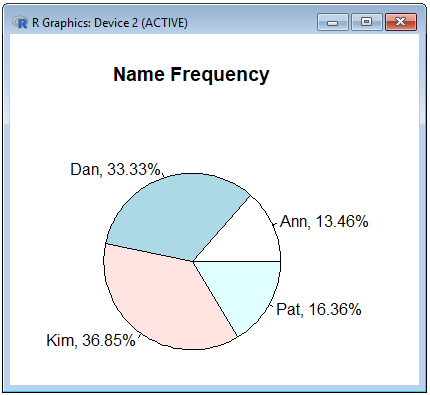
Show the proportions as a pie chart.
perc = paste(round(100*ft$p,2), "%", sep="")
lbls = paste(ft$fn, perc, sep=', ')
pie(ft$p, labels=lbls, main='Name Frequency')
Function paste() is used here to format and combine names and proportions into labels incorporated onto the chart.
It works like Excel's function =CONCATENATE().
This is it!
The real power of R lies in handling external data sources. In addition to those listed above, R can also accept input from a keyboard. Function readline(prompt = "") can do this job. The prompt argument is an invitation to provide an input. The following example imitates a simple game: Rolling a Die. The entire code is wrapped up in a [user-defined] function, check_roll(). When function is called, it is provided with a randomly generated number, selected from a set of numbers (1,2,...,6), stored in variable die. It is done, using function sample() that takes the set (here die)and randomly selects one number from it. The selection is done according to an uniform distribution. An alternative generator would be: ceiling(runif(1, min=0, max=6)).
check_roll = function(roll) {
guess = readline('Your guess: ')
guess = as.integer(guess)
if (guess == roll)
cat('Go it!\n')
else
cat('Sorry, the roll result is:',roll,'\n')
}
if( interactive() ) check_roll( sample(1:6,1) )
Your guess: 6
Sorry, the roll result is: 4
Copyright © 2019 biiat.com
Contributed by Nicholas Letkowski.