Transportation Problems
Problem Statement
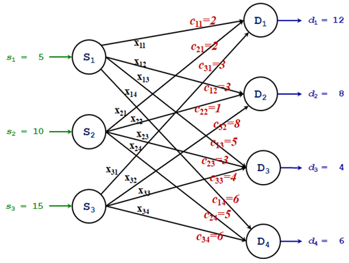
There are m = 3 suppliers and n = 4 destinations (points of demand). The sources are labeled as S1, S2, ..., Sm. The destination are labeled as D1, D2, ..., Dn. Each of the suppliers (S1, S2, ..., Sm) can ship goods to each of the consumers (D1, D2, ..., Dn), at a fixed unit transportation cost, cij, i = 1,2,...,m; j = 1,2,...,n. Decision variables xij, i = 1,2,...,m; j = 1,2,...,n, are the quantities of goods shipped from the suppliers to the consumers. The following models shows this problem graphically and mathematically:
 |
Decision Goal,
Minimize:
Z = 2x11 + 3x12 + 5x13 + 6x14 +
2x21 + 1x22 + 3x23 + 5x24 +
3x31 + 8x32 + 4x33 + 6x34
Supply Constraints:
x11+x12+x13+x14 = 5
x21+x22+x23+x24 = 10
x31+x32+x33+x34 = 15
Demand Constraints:
x11+x21+x31 = 12
x12+x22+x32 = 8
x13+x23+x33 = 4
x14+x24+x34 = 6
Variable Limit Constraints:
All xij ≥ 0 |
| Figure 1. A graphical model for a transportation problem. | |
This is a balanced problem, meaning that the total supply is equal to the total demand. A feasible solution is a combination of the non-negative shipments that exhaust the supply and satisfy the demand (meet the constraints). The optimal solution is a feasible solution that fulfills the decision goal.
Finding a Feasible Solution with the North-West Corner Method
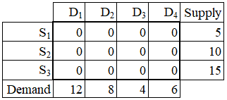
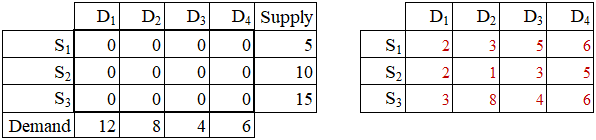
It will be more convenient to present the problem in form of the X matrix, representing the decision variables plus two vectors, defining the supply and demand quantities. Initially, the decision variables are all set to zero (no shipment). The supply and demand quantities are at their original levels.
Initialization:
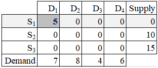
Step 1: For the upper-left most (North-West) cell, S1→D1, ship as much as possible from S1 to D1. Since S1 has 5 units and D1 wants 12 units, only 5 units are shipped. The S1 supply quantity is exhausted and D1 demand quantity remains at level 7 = 12 - 5.
The set and update operations are:
x11 = min(s1, d1) = 5
s1 := s1 - x11 = 0
d1 := d1 - x11 = 7
Notice that notation := stands here for an update operation. It means that the new value of the left-hand side variable uses its old value that appears in the right-hand side expression.
Since S1 has no more supply, it is eliminated from further processing (this is signified by shading row S1).
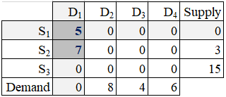
Step 2: The next North-West Corner route is cell S2→D1. Ship as much as possible from S2 to D1. Since S2 has 10 units and D1 wants 7 units, the quantity shipped is 7. The D1 demand is already satisfied and S2 supply remains at level 3 = 10 - 7.
The set and update operations are:
x21 = min(s2, d1) = 7
s2 := s2 - x21= 3
d1 := d1 - x21= 0
Since D1 is fully satisfied, it is eliminated from further processing.
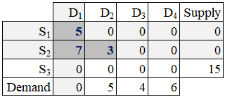
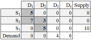
Step 3: After elimination of row 1 (S1) and column 1 (D1), the upper-left (NWC) route is cell is S2→D2. Ship as much as possible from S2 to D2. Since S2 has 3 units and D2 wants 8 units, the quantity shipped is 3. The S2 supply quantity is exhausted and D2 demand quantity remains at level 5 = 8 - 3.
The set and update operations are:
x22 = min(s2, d2) = 3
s2 := s2 - x22 = 0
d2 := d2 - x22 = 5
Since S2 is fully commited, it is eliminated from further processing.
Step 4: At this stage, the upper-left (NWC) route is cell is S3→D2. Ship as much as possible from S3 to D2. Since S3 has 15 units and D2 wants 5 units, the quantity shipped is 5. The D2 demand is fully satisfied and S3 supply quantity remains at level 10 = 15 - 5.
The set and update operations are:
x32 = min(s3, d2) = 5
s3 :=s3 - x32 = 10
d2 := d2 - x32 = 0
Since D2 (column 2) is fully satisfied, it is eliminated from further processing.
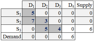
Step 5: The current NWC route is cell is S3→D3. Ship as much as possible from S3 to D3. Since S3 has 10 units and D3 wants 4 units, the quantity shipped is 4. The D3 demand quantity is fully satisfied and S3 supply quantity remains at level 6 = 10 - 4.
The set and update operations are:
x33 = min(s3, d3) = 4
s3 := s3 - x33= 6
d3 := d3 - x33 = 0
Since demand D3 (column 3) is fully satisfied, it is eliminated from further processing.
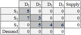
Step 6: There is only one route left over. It is cell is S3→D4. Since this transportaion problem is balanced, the remaining supply and demand quantities are equal. S3 has 6 units and D3 wants 6 units. The quantity shipped is 6. The D4 demand quantity is fully satisfied and S3 supply quantity is exhausted (0 = 6 - 6).
The set and update operations are:
x34 = min(s3, d4) = 6
s3 :=s3 - x34 = 0
d4 := d4 - x34 = 0
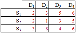
Since demand D4 (column 4) is fully satisfied, and supply S3 (row 3) is fully committed, both the entities are closed and the problem is solved. For convenience, the unit transportion cost matrix is also shown.
The total transportation cost for this [feasible] solution is equal 2*5 + 2*7 + 1*3 + 8*5 + 4*4 + 6*6 = 119.
Challenge 1
Automate this procedure in Excel. Use the following start up workbook:
nwc_method.xlsm.
Challenge 2
Automate this procedure (NWCM) in R. Use the following vectors to set supply (s), demand (d), and unit transportion costs (utc):
s = c(5,10,15)
d = c(12,8,4,6)
utc = c(2,3,5,6,2,1,3,5,3,8,4,6)
Finding a Feasible Solution with the Minimum Cost Method
This method selects shipping routes that have the lowest unit transportation cost so far. The initial state has no shipments and all routes are available.
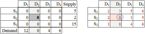
Step 1: Select a cell (route) that has the lowest unit-transportation cost (utc). At this initial stage, the minimum utc is located in cell S2→D2(the new circled value, shown in the following image). Ship as much as possible from S2 to D2. Since S2 has 10 units and D2 wants 8 units, the quantity shipped is 8. The D2 demand quantity is fully satisfied and S2 supply quantity remains at level 2 = 10 - 8.
The set and update operations are:
x22 = min(s2, d2)
s2 := s2 - x22
d2 := d2 - x22
Since D2 is fully statisfied, it is eliminated from further processing (this is signified by shading column D2).
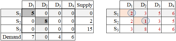
Step 2: Again, select a cell (route) that has the lowest unit-transportation cost (utc). There are two cells having the lowest utc. In this tied situation, we can make the selection arbitrarily. Let's pick cell S1→D1(the new circled value, shown in the following image). Ship as much as possible from S1 to D1. Since S1 has 5 units and D1 wants 12 units, the quantity shipped is 5. The S1 supply quantity is exhausted and D1 demand quantity remains at level 7 = 12 - 5.
The set and update operations are:
x11 = min(s1, d1)
s1 := s1 - x11
d1 := d1 - x11
Since supply S1 is exhausted, it is eliminated from further processing (this is marked up by shading row S1).
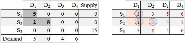
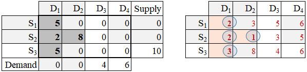
Step 3: The next lowest unit-transportation cost (utc) is located in cell S2→D1. Ship as much as possible from S2 to D1. Since S2 has 2 units and D1 wants 7 units, the quantity shipped is 2. The S2 supply quantity is exhausted and D2 demand quantity remains at level 5 = 7 - 2.
The set and update operations are:
x21 = min(s2, d1)
s2 := s2 - x21
d1 := d1 - x21
Since supply S2 is exhausted, it is eliminated from further processing (this is marked up by shading row S2).
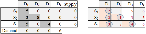
Step 4: The next lowest unit-transportation cost (utc) is located in cell S3→D1. Ship as much as possible from S3 to D1. Since S3 has 15 units and D1 wants 5 units, the quantity shipped is 5. The D1 demand quantity is fully satisfied and S3 supply quantity remains at level 10 = 15 - 5.
The set and update operations are:
x31 = min(s3, d1)
s3 := s3 - x31
d1 := d1 - x31
Since demand D1 is fully statisfied, it is eliminated from further processing (this is signified by shading column D1).
Step 5: The next lowest unit-transportation cost (utc) is located in cell S3→D3. Ship as much as possible from S3 to D3. Since S3 has 10 units and D3 wants 4 units, the quantity shipped is 4. The D3 demand quantity is fully satisfied and S3 supply quantity remains at level 6 = 10 - 4.
The set and update operations are:
x33 = min(s3, d3)
s3 := s3 - x33
d3 := d3 - x33
Since demand D3 is fully statisfied, it is eliminated from further processing (this is signified by shading column D3).
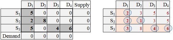
Step 6: The final lowest unit-transportation cost (utc) is located in cell S3→D4. Ship as much as possible from S3 to D4. Since S3 has 6 units and D4 wants 6 units, the quantity shipped is 6. The D4 demand quantity is fully satisfied and S3 supply is exhausted.
The set and update operations are:
x34 = min(s3, d4)
s3 := s3 - x34
d4 := d4 - x34
Since demand D4 (column 4) is fully satisfied, and supply S3 (row 3) is fully committed, both the entities are closed and the problem is solved.
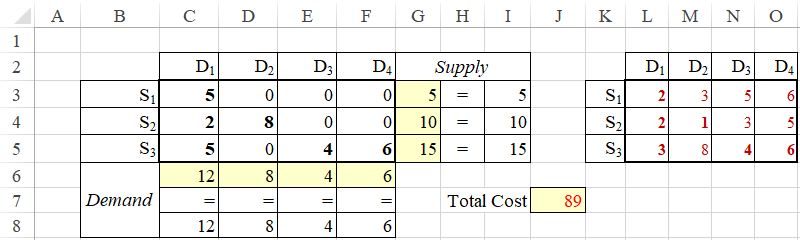
The total transportation cost for this [feasible] solution is equal 2*5 + 2*2 + 1*8 + 3*5 + 4*4 + 6*6 = 89.
Challenge 3
Automate this procedure in Excel. Use the following start up workbook:
mc_method.xlsmChallenge 4
Automate this procedure (MCM) in R. Use the following vectors to set supply (s), demand (d), and unit transportion costs (utc):
s = c(5,10,15)
d = c(12,8,4,6)
utc = c(2,3,5,6,2,1,3,5,3,8,4,6)
Finding an Optimal Solution
Notice the the Minimum Cost Method shown above provided [coincidently] the same solution.
Use the following code to solve this problem in R.
install.packages("linprog") # Skip it if this package is already installed.
library(linprog)
s = c(5,10,15) # Supply
d = c(12,8,4,6) # Demand
utc = c(2,3,5,6,2,1,3,5,3,8,4,6) # Unit Transportation cost
m = length(s)
n = length(d)
C = matrix(utc, nrow=m, ncol=n, byrow=TRUE)
sr = rep("=",m)
dr = rep("=",n)
optX = lp.transport( cost.mat=C, direction="min", row.signs=sr, row.rhs=s, col.signs=dr, col.rhs=d )
optX
Success: the objective function is 89
X = optX$solution
colnames(X) = paste("D", 1:n, sep="")
rownames(X) = paste("S", 1:m, sep="")
X
   D1 D2 D3 D4
S1  5  0  0  0
S2  2  8  0  0
S3  5  0  4  6
This is it!