Programming Cases
The Economic Order Quantity model is one of the oldest mathematical model for solving a simple inventory management problem, involving fixed and uniform demand. It was developed by Ford W. Harris in 1913 [1].
The model has just one decision variable, Q, representing the order quantity, and the following model parameters:
D – annual demand,
c – fixed setup cost of one-time order (order handling cost),
h – annual unit holding cost per inventory item,
y – the length of the year in days.
There are D/Q orders, each incurring a cost of c dollars. The highest inventory level is Q and the lowest—zero. Since demand is uniformly distributed, the average inventory level is Q/2 = (0 + Q)/2. Thus, the average holding cost is h · Q/2. Putting the two costs together, the average inventory cost (annually) is given by the following function:
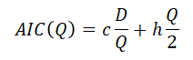
The optimal solution (order quntity) is a Q* value that minimizes the average inventory cost, AIC(Q*):
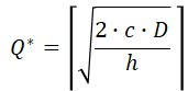
Notation ⌈ ⌉ stands here for rounding up to the nearest integer.
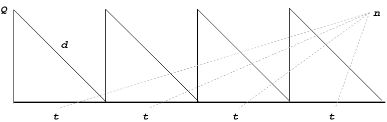
Additional characteristics of this model are:
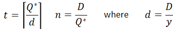
t - the length of the single inventory cycle,
n - the number of the inventory cycles
t - the length of the single inventory cycle,
n - the number of the inventory cycles
The t and n parameters are calculated as follows:
Develop a Python application that will print the following report:
- The optimal solution, Q*. In Python use variable name optQ.
- The average inventory cost for the optimal solution, AIC(Q*) (variable name aic).
- The length of the inventory cycle for the optimal solution (variable name t).
- The number of the inventory cycles for the optimal solution (variable name n).
Test your application for the following data:
- Variable D = 4320
- Variable c = 10.0
- Variable h = 4.8
- Variable y = 360
Round up the optimal solution and the cycle, t, value to an integer (use the math.ceil fucntion). Adjust the optimal solution so it will be a multiple of the daily demand value (d). Recalculate the average annual inventory cost for the new Q*value.
References
| [1] | Letkowski, J. (2018). Decision models for the newsvendor problem – learning cases for business analytics, Journal of Instructional Pedagogies, Volume 21 (), AABRI Academic Journals - JIP. Manuscript. |